

Understanding how stock market returns behave is crucial for investors and traders. One of the most important statistical tools used to model price behavior and risk is the normal distribution. This blog will explain what a normal distribution is, how it helps us estimate probabilities of price movements, why we use log returns instead of simple returns in financial modeling, and how we’ve applied all of this to real Nifty 50 daily return data from FY 2024–25.
What is a Normal Distribution?
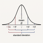
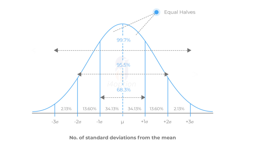
A normal distribution, or bell curve, is a symmetrical, continuous probability distribution centered around its mean. It describes how data values are expected to spread out: most data points cluster around the average (mean), and fewer appear as you move away from it in either direction.
Key Properties:
- It’s symmetrical about the mean.
- The mean, median, and mode are all the same.
- It’s fully described by two parameters:
- μ (mu): the mean
- σ (sigma): the standard deviation
What is the Normal (Gaussian) Probability Function?
The normal distribution probability function, also called the Gaussian Probability Density Function (PDF), describes the shape of the bell curve and the density of values around the mean.
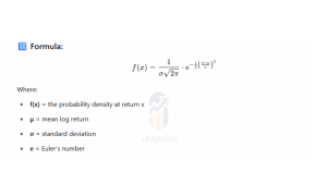
Where:
- f(x) = the probability density at return x
- μ = mean log return
- σ = standard deviation
- e = Euler’s number
- π = Pi
This function gives you the relative likelihood of seeing a specific return. It’s highest at the mean and tapers off as returns deviate further. The area under the curve = 1, representing total probability.
Used to visualize how returns are distributed, but not to calculate the probability between ranges — for that, we use the cumulative version below.
Why Use Log Returns Instead of Simple Returns?
In financial modeling, we use logarithmic returns (log returns) instead of simple returns because:
- Time-Additivity: Log returns can be added across periods.
- Better Normality: They more closely resemble a normal distribution.
- Compounding Compatibility: They represent continuous growth more accurately.
- Statistical Consistency: Many financial models (e.g., Black-Scholes) assume log returns.
In this analysis, we’ve used the “Log Return” column from Nifty 50 daily data. All mean and standard deviation calculations, as well as probability estimates, are based on this.
How to Calculate Probability for a Range
To calculate the chance of returns staying within a certain range (e.g., -1% to +1%), we use the Cumulative Distribution Function (CDF) of the normal distribution:
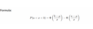
Where:
- Φ = CDF of normal distribution
- μ = mean log return
- σ = standard deviation of log returns
- a, b = lower and upper bounds of return range
This gives you the probability that a return falls between a and b on any given day.
Real-World Example Using Nifty 50 Log Returns
We analyzed Nifty 50 daily log returns from April 1, 2024 to March 31, 2025. Using the calculated mean and standard deviation, we estimated the chance that daily returns would stay within specific ±% ranges.
| Range (±%) | Lower Bound | Upper Bound | Probability (%) |
|---|---|---|---|
| ±0.50% | -0.0050 | 0.0050 | 42.73 |
| ±1.00% | -0.0100 | 0.0100 | 74.08 |
| ±1.50% | -0.0150 | 0.0150 | 90.94 |
| ±1.75% | -0.0175 | 0.0175 | 95.17 |
| ±2.00% | -0.0200 | 0.0200 | 97.60 |
Interpretation:
- There’s a 42.7% chance Nifty’s daily return stays within ±0.5%
- A 74% chance for ±1% movement
- A 97.6% chance of remaining within ±2% on any given day
These stats help traders set realistic stop-losses, targets, and option pricing levels.
Important point: all calculations performed are on the Nifty 50 daily close value, which is important for all types of traders, but you can extend this research to day range also. means you can find the probability of the day range of Nifty ( day low to high ).
You can calculate any range probability, and also extend your data sample size. to get this Excel template, send a message on WhatsApp: Get file
Visualizing the Nifty 50 Log Return Distribution
Below is a chart of actual Nifty 50 daily log returns vs the ideal normal distribution:
Distribution of Nifty 50 Log Returns with Normal Curve Overlay
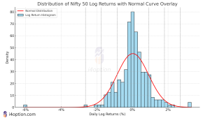
What the Chart Shows:
- Blue bars = Actual return frequency
- Red curve = Ideal bell curve based on mean & std dev
- Dashed lines = ±1σ, ±2σ, ±3σ boundaries
You can observe that:
- Most data clusters near 0%
- The tails are slightly fatter than a perfect normal, which is common in financial returns (more extreme days than expected)
Final Thoughts: How Useful is the Normal Distribution?
The normal distribution is a powerful framework to estimate market behavior, used widely in:
- Risk management (e.g., Value at Risk)
- Option pricing models (e.g., Black-Scholes)
- Trade planning (e.g., setting realistic stop-losses)
- However, markets aren’t perfectly normal — they show skew and fat tails during volatile periods.
Still, for typical daily behavior, assuming a normal distribution is a great start — especially for indices like Nifty 50 with high liquidity and diversified components.
Coming Up Next…
In our next blog, we’ll explore:
- 📊 Log returns vs simple returns: What’s the real difference?
- 🚨 Fat tails and black swan events: Why markets surprise us
- 🧮 Probability functions & Alternative distributions: t-distributions, skew-normal, etc.
📢 If you found this helpful, share it with fellow traders at blog.i4option.com