What is a Continuous Function?

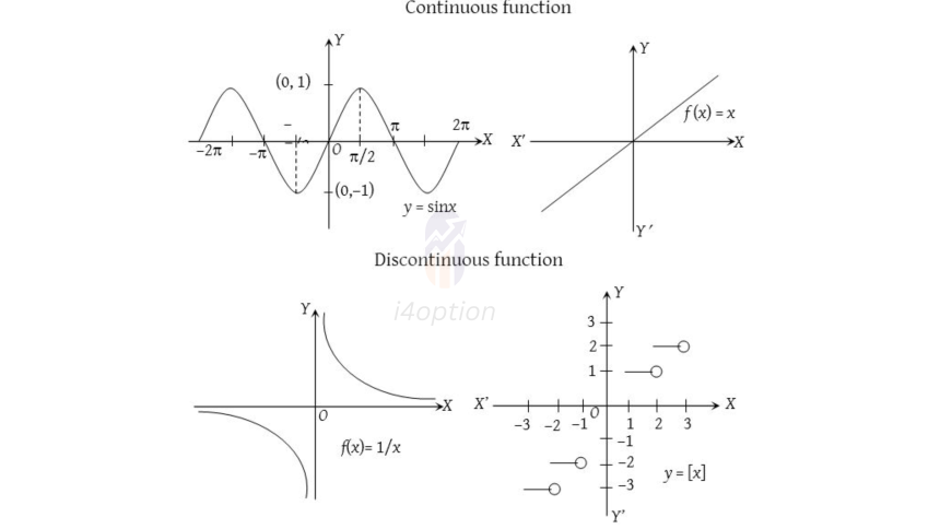
In mathematics, a continuous function is a function you can draw without lifting your pencil from the paper. Intuitively, this means the function’s output changes smoothly as the input changes, with no sudden jumps or gaps. More formally, for a function to be continuous, a tiny change in the input causes only a tiny change in the output – there are no abrupt breaks. If you imagine the graph of a continuous function, it’s an unbroken curve.

Real-Life Examples of Continuous Data: Many quantities we encounter are continuous by nature, meaning they can take on any value in some range (often including fractional or decimal values):

• Temperature: It doesn’t jump from 20°C to 21°C in one tick; it passes through all intermediate values (20.1, 20.2, …) smoothly. A day’s temperature is a continuous function of time.
• Time: Time flows continuously. We can measure time in hours, minutes, seconds, or infinitely small fractions of a second.
• Distance: If you drive from point A to B, your distance from A increases continuously – you don’t teleport from 1 km to 2 km. Every fraction in between was covered.
• Height of a Person or Horse: Height can be 5 feet, 5.5 feet, 5.501 feet, etc. – any value within a plausible range.

In each case, any fractional value is meaningful. Between any two different continuous values, there are infinitely many other possible values. Contrast this with discrete examples (like counts of people or objects) where only specific separate values make sense – we’ll get to that in the next part of the series.

Continuous Functions in Finance: Finance has many concepts that are modeled as continuous functions or continuous processes:

• Stock Prices Over Time (idealized): If we treat the price of a stock as a function of time, we often model it continuously. In calculus-based models, a stock’s price S(t)  changes smoothly with time t (even though in reality, tick-by-tick movements are tiny discrete jumps). For example, the famous Black-Scholes option pricing model assumes stock prices follow a continuous path (a Brownian motion model). This is a useful approximation because it makes the math workable, even if real prices have minuscule jumps.
• Continuous Compounding of Interest: Interest can be compounded discretely (e.g., yearly or monthly) or continuously. Continuous compounding assumes interest is added in an infinitely small, continuous way. The formula for continuous compounding is  FV=\(Pe^{rt}\), meaning an initial principal P grows at rate r continuously over time t. This formula comes from taking the limit as compounding periods become very frequent. Continuous compounding yields a slightly higher return than discrete compounding at the same nominal rate. For instance, at 10% annual interest, continuous compounding would turn ₹100 into ₹110.5 in one year (versus ₹110.00 with once-yearly compounding). The continuous growth is a smooth exponential curve, as opposed to step-wise jumps on compounding dates.
• Probability Distributions: Some key probability models in finance are continuous functions. The normal distribution (the bell curve used for asset returns) is defined by a continuous probability density function. You can plug any value into a normal distribution’s formula and get a density – the distribution is smooth and unbroken across all real numbers.

Analogy – Water Flow vs. Counting: A continuous function is often compared to a flowing stream of water. Water can be measured in any amount: 1 liter, 1.5 liters, 1.234 liters, etc. In finance, think of something like the time value of money accruing continuously – value drips and accumulates every instant. This is different from a discrete scenario like counting coins, where you have whole units and nothing in between.

In summary, continuous functions let us model gradual change. They’re incredibly useful in finance for theoretical models and calculations. While the real world might be granular at a micro level, treating things as continuous often makes analysis easier and is a good approximation when changes are frequent or increments are very small.

What is a Discrete Function?

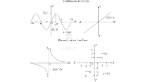
A discrete function is essentially the opposite of continuous – it’s defined only at specific, separated input values, rather than for every value in an interval. You can think of a discrete function as one that jumps from point to point with nothing in between. If you tried to draw its graph, you would lift your pencil between plotted points, because there are gaps. In a discrete dataset, values are distinct and not connected on a continuum.

Plain English Definition: A discrete function allows the input (and often the output) to be only certain specific values, usually integers or counts. Any values between those specific points either don’t exist or don’t make sense for that function.

Real-Life Examples of Discrete Data:

• Counting People or Objects: You can have 3 people in a room or 4 people, but not 3.5 people. The number of people is a discrete variable (typically only whole numbers). The function “population over time” would jump whenever a person enters or leaves – it’s not a smooth curve.
• Shoe Sizes: Often, shoe sizes are in discrete steps (say, full and half sizes). If a brand only makes sizes 8 and 9, size 8.5 might not exist in that system.
• Monthly Profit: If a business calculates profit month by month, you might consider profit as a discrete function of month number (January, February, etc.). You only evaluate it once per month, not for every day in between, if you’re strictly using monthly snapshots.
• Dividends Paid by a Stock: Many companies pay dividends quarterly. If you plot dividends over time, you get spikes every 3 months and zero in between – a discrete series of cash flows rather than a continuous trickle.

In these cases, in-between values are not defined or are not meaningful. For example, it doesn’t make sense to talk about the “number of TV sets in a home” as 2.5 – it has to be 2 or 3, etc.. If you graphed “TV sets per household” for different households, you’d just have separate points (e.g., a lot of 1’s and 2’s, maybe some 0 or 3) with no values like 1.7 in between.

Discrete in Finance – Key Examples: Finance and trading have plenty of discrete elements, even though we often approximate them as continuous for modeling convenience:

• Stock Prices (Tick Size): On many exchanges, stock prices move in minimum increments (ticks). For example, in our markets, prices are typically quoted in 5 paisa ticks. A stock price can be ₹100.00 or ₹100.05, but not ₹100.004 because ₹0.05 is the smallest tick size. In this sense, stock prices are a discrete variable – they snap to a penny grid. Meanwhile, if you convert that price change into a return percentage, the return can be any real number, making returns continuous. But the price itself has discrete granularity. ( To be noted here, though most of the stocks and derivatives we trade have a .5 tick size, but some stocks have .1, i.e, 1 paisa tick size, so no need to confuse if I use .5 or write .o1 tick size)
• Trading in Whole Units: When you buy stocks, you usually buy whole shares (1 share, 2 shares, 100 shares, etc.). In our Indian market, as well as many markets our the globe, you cannot buy 2.7 shares – share count is discrete. (Fractional shares have become more common recently for small investors, but even fractional shares usually break ownership into very fine, discrete units behind the scenes.)
• Accounting Figures:  Counts of things like the number of trades, the number of employees at a firm, or the days until a futures contract expires are all discrete numbers. For example, if you track how many trades you made each day this week, you might have a function like
  $f$ 

  (day)=number of trades. If on Monday you made 5 trades and on Tuesday 8 trades, there’s no meaning to $f(\text{Monday afternoon})$ 

  unless you break the day further – at daily resolution, the function jumps from 5 to 8.

• Binomial Outcomes in Trading: Consider a simple trading strategy that either “wins” or “loses” each day (say, ends the day with a profit or a loss). We can model each day’s outcome as a discrete variable (profit vs. loss, or +1 vs. 0 in a simplified model). Over a week of 5 trading days, the total number of winning days is described by a discrete function (it can be 0, 1, 2, … up to 5). This is essentially following a binomial distribution, which is discrete.

In practice, discrete functions often appear when dealing with counts (how many?) or specific intervals (this day, that day). They’re crucial in situations like option pricing with binomial trees, where time is broken into discrete steps and the stock is assumed to either go up or down in each step. Each step is like a discrete function of time.

Takeaway: A discrete function breaks things into clear-cut steps or counts. In trading, even though underlying phenomena like price movement feel continuous, the measured values can be discrete (due to price ticks, trading only happening at discrete times, etc.). Understanding discrete vs. continuous is important because it affects how we model and calculate probabilities. For some problems, a discrete model (counting successes or failures, like coin flips or up/down days) is appropriate; for others, a continuous model (like assuming returns vary along a smooth distribution) fits better. Recognizing the discrete nature of some financial variables keeps our models realistic when needed – you can’t have half a trade or a stock at half a penny (on most exchanges) without special conditions.

Is the Stock Market a Continuous or Discrete System?

This is a fascinating question because the stock market has elements of both. The answer depends on perspective and context. Let’s explore both sides:

Discrete Aspects of the Market

On a fundamental level, many actions in the stock market happen in discrete steps:

• Price Changes in Ticks: Stock prices change in discrete increments (ticks). For example, if the minimum price increment is ₹0.05, a stock can move from ₹100.00 to ₹100.05, but not ₹100.005 in actual trading. This suggests price levels are discrete grid points.
• Trades at Discrete Times: Trades occur at specific timestamps. Even with high-frequency trading, each transaction is a separate event. Time is often treated in intervals (seconds, milliseconds, etc.) for analysis. You might say that trades are coming in continuously during market hours, but really, there’s a countable (albeit large) number of trades each day, each at a precise time. Outside of market hours, no trading occurs in most markets, introducing clear breaks.
• Data Feeds and Candles: Market data is recorded in discrete intervals for practical use – e.g., 1-minute candles, daily closing prices. Indicators and charts often use these discrete time slices.
• Financial Statements and Events: Fundamental events like earnings reports happen discretely (usually quarterly). Corporate actions (dividends, splits) occur on specific dates, not continuously.

These realities mean that if you zoom in, the market is naturally discrete – a sequence of individual transactions and price quotes. In fact, from a strict viewpoint, stock prices have a discrete state space and (during normal hours) a discrete time sequence. One can argue that stock market data is a “discrete-time, discrete-state” process at the very granular level (price jumps by ticks at distinct event times).

As an example, consider binomial models for stock prices: They assume that in each small time step, the price either moves up or down by a certain amount (a discrete change). This is a discrete approximation of how prices evolve, and such models can be very useful in option pricing and scenario analysis.

Continuous Aspects of the Market

Despite the discrete nature of individual trades, modeling the market as a continuous system has great appeal and practical value:

• Continuous-Time Models: In finance theory, we often treat time as a continuum. Models like the Black-Scholes option pricing formula assume stock prices follow a continuous-time stochastic process (Geometric Brownian Motion). In these models, S(t) (the stock price) exists for every moment t≥0, not just at trading instants. This yields elegant math and closed-form solutions. In reality, you can’t observe the price at every fraction of a second, but the model supposes you could.
• Continuous State (Price) Models: Even though price quotes have ticks, we could conceptually imagine a world where tick size is infinitesimally small (or zero). In fact, currencies and some assets can be quoted in very fine fractions, and if we let the tick size go to zero in theory, the price becomes a continuous variable. Many mathematical results (like calculus-based tools) treat price as moving through real numbers smoothly. It’s an approximation, but a useful one. As one quantitative finance discussion noted, “we can model stock prices as a time and space continuous process… continuous models are often limits of the discrete models”. This means a continuous model can be seen as what happens when discrete steps become extremely small and numerous.
• Interpolation of Data: Even though trades are discrete, we often interpolate to create continuous charts (think of a line chart connecting price points). If you look at a stock chart, it appears as a continuous line. We mentally treat that line as if the price existed at every point along it, even though it’s drawn from discrete samples.
• Analogy to Physics: Just like matter is atomic (discrete) but we often model it as continuous (like treating a solid object as a continuous mass in physics), stock prices might be inherently tick-by-tick, yet treating them as continuous allows the use of calculus and differential equations to model trends, volatility, and option Greeks.

Reconciling the Two Perspectives

In truth, both views are valid and they complement each other. The discrete view is closer to the literal truth of market mechanics (trades and ticks), while the continuous view is a mathematical idealization that makes analysis tractable. One could say, stock prices are a continuous process that we observe discretely, or conversely that they are discrete by nature but well-approximated by continuous models. As one expert quipped, whether stock prices are continuous or discrete “is almost a philosophical question”.

Think about very active markets with tiny tick sizes (like foreign exchange with pip increments, or liquid stocks). The price changes so frequently and in such small amounts that, for many purposes, it’s practically continuous. On the other hand, in a stock with low liquidity, you might literally see it jump from ₹10 to ₹10.5 with no trades in between – a clearly discrete jump.

When building models:

• For short-term, high-precision tasks (like algorithmic trading or exchange microstructure analysis), a discrete approach (down to each trade or quote change) is important.
• For long-term, macro-level modeling (like portfolio theory, Black-Scholes pricing, risk calculations), continuous models are preferred for their mathematical convenience and insight, acknowledging that in implementation, one will eventually discretize (e.g., simulate at small time steps on a computer, since continuous math still needs to be approximated digitally).

Example: The Binomial option pricing model (discrete-time) versus the Black-Scholes model (continuous-time) illustrates this dichotomy. The binomial model uses a step-by-step process (e.g., every Δt period the stock moves up or down by a factor). If you increase the number of steps and shrink each step’s size, the binomial model’s price will converge to the Black-Scholes price. In other words, continuous is the limit of discrete in this case.

Bottom Line: The stock market can be viewed as discrete in reality but often treated as continuous in theory. Understanding both perspectives gives a trader or analyst flexibility. We know the market operates in ticks and trades (discrete events), but we often analyze it with smooth curves and calculus. It’s much like viewing light as particles vs. waves – use the perspective that best solves the problem at hand, while remembering the limitations of each view.

If you like these data analytical blogs, do share, and if any queries, don’t hesitate to ask in the comments section.