

Abstract:
In the dynamic and uncertain landscape of financial markets, probability distribution functions serve as indispensable tools for quantitative analysis and risk management. This report provides a comprehensive overview of the most commonly employed probability distributions—Normal, Lognormal, Binomial, Poisson, and Student’s t—detailing their core characteristics, practical applications, and inherent limitations within the context of institutional trading and high-frequency trading (HFT) operations. Drawing upon illustrative examples from Indian markets, such as the Nifty 50, Bank Nifty, and individual stocks like TCS and Reliance Industries, the analysis underscores how these mathematical constructs enable traders to quantify uncertainty, evaluate strategies, and manage exposure to extreme market events. The discussion highlights the critical evolution of modeling approaches, from foundational assumptions to more sophisticated hybrid methodologies, emphasizing the continuous adaptation required to navigate the complexities of real-world financial data.
Introduction: Quantifying Uncertainty in Financial Markets
The financial markets are inherently probabilistic, characterized by constant fluctuations and unpredictable events. For any participant, from retail traders to sophisticated institutional desks, navigating this environment necessitates a robust framework for quantifying uncertainty. This is precisely where probability distribution functions become central. A probability distribution is fundamentally a mathematical construct that describes the likelihood of various outcomes for a random variable. For instance, analyzing the distribution of daily returns for a benchmark index like the Nifty 50 or a prominent stock such as TCS provides critical insights into the probable range of future price movements and the likelihood of different return values.
Effective trading strategies are not built on certainties but on a nuanced understanding of probabilities. The ability to estimate the chances of profits or losses, anticipate extreme price shifts, or predict the frequency of specific market events empowers traders to make more informed decisions regarding risk exposure and strategic positioning. This approach shifts the focus from a single expected outcome to a spectrum of possible outcomes, each with an associated probability, which is a hallmark of professional trading.
This report will introduce these key probability distribution functions, emphasizing those most commonly utilized by institutional traders, high-frequency trading algorithms, and professional trading desks. To ground these theoretical concepts in practical reality, numerous examples from the Indian markets, including the NSE and BSE, will be employed, illustrating their application to indices like the Nifty 50 and Sensex, and individual stocks such as TCS, RIL, etc. While the Bernoulli distribution (for binary outcomes) is foundational, the focus will be on the Binomial, Poisson, Normal, Lognormal, and Student’s t-distribution, alongside other heavy-tailed distributions that capture the nuances of market behavior.
Probability Functions: Discrete vs Continuous
A probability function (also known as a probability distribution function) is a mathematical rule that describes the likelihood of different outcomes for a random variable. It provides a complete picture of all possible values the random variable can take, along with the probability associated with each value. All probabilities defined by such a function must be non-negative, and the total probability across all outcomes sums (or integrates) to 1.
There are two main categories of probability distributions, depending on whether the random variable is discrete or continuous:
- Probability Mass Function (PMF): Used for discrete random variables that can only take on a finite or countably infinite set of values (e.g. the result of rolling a die, or the number of winning trades out of 10). The PMF, often denoted P(X = x), gives the probability that the random variable X equals a specific value x.
- Key properties: Every probability P(X = x) ≥ 0, and the sum of probabilities over all possible values equals 1.
- Examples: The Binomial distribution (models the number of successes in a fixed number of independent trials), Poisson distribution (number of events occurring in a fixed interval), Geometric distribution (number of trials needed to get the first success), etc.
- Probability Density Function (PDF): Used for continuous random variables that can take on any value in a range (e.g. an asset return or price, which can vary in a continuous spectrum). For a continuous variable, the probability of it taking an exact single value is 0 – instead, we use the PDF, denoted f(x), to find the probability that the variable falls within a range of values.
- Key properties: f(x) ≥ 0 for all x, and the total area under the density curve is 1 (i.e. ∫_{-∞}^{∞} f(x) dx = 1).
- Examples: The Normal distribution (Gaussian) – a symmetric “bell curve” defined by a mean and standard deviation, Uniform distribution (all outcomes in a range equally likely), Exponential distribution (models waiting times between Poisson events), etc.
In trading, both discrete and continuous distributions are useful. For example, whether a single trade is profitable can be treated as a discrete (0/1) outcome, whereas daily price returns are usually modeled as continuous variables. Next, we’ll explore the specific distributions most used in trading and how traders leverage them.
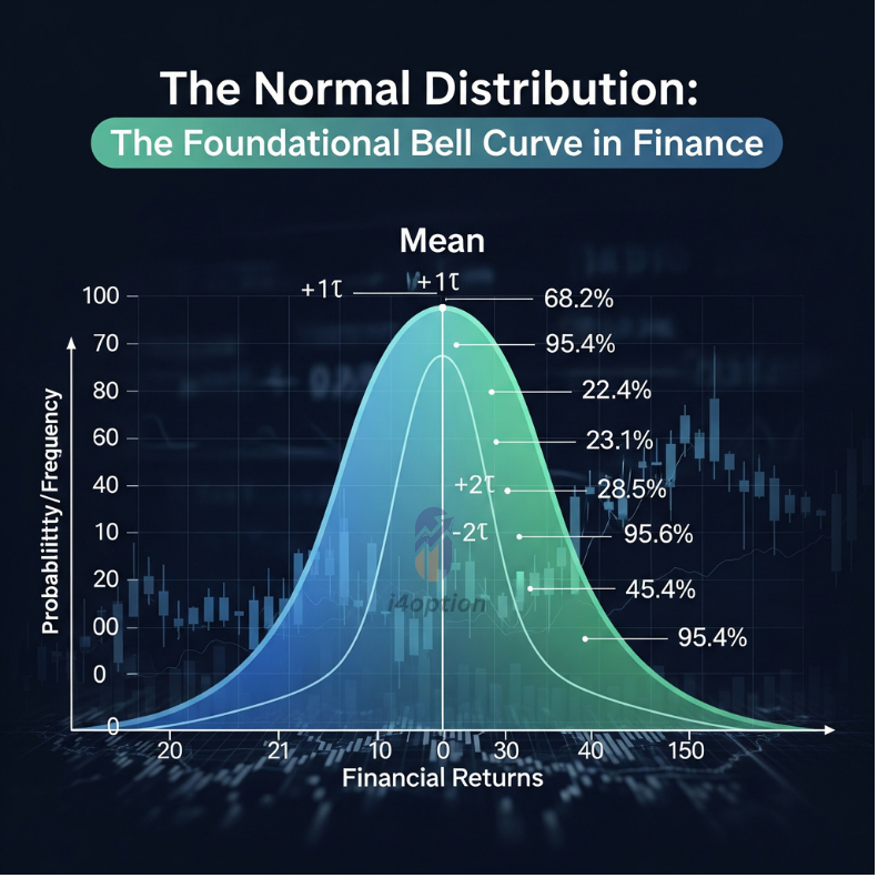
1. The Normal Distribution: The Foundational Bell Curve in Finance
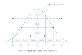
The normal distribution is a symmetric, bell-shaped curve characterized by its mean (average) and standard deviation (volatility). It often underpins models of price changes and returns in markets due to the Central Limit Theorem (loosely speaking, the sum of many small random effects tends to be normally distributed). Traders commonly assume daily returns are roughly normal as a first approximation. For example, if we look at the daily percentage change of the Nifty 50 index or a stock like TCS, the bulk of those daily moves cluster around the average, with fewer days exhibiting very large moves. Under a normal distribution assumption, we can use the well-known “68–95–99.7 rule” (empirical rule) to understand volatility: roughly 68% of outcomes fall within 1 standard deviation (σ) of the mean, ~95% within 2σ, and ~99.7% within 3σ.
Standard normal distribution illustrating the “68–95–99.7” empirical rule: ~68% of outcomes lie within ±1σ of the mean, ~95% within ±2σ, and ~99.7% within ±3σ.Traders often rely on this bell curve model to set expectations. For instance, if Nifty 50’s daily volatility (σ) is ~1%, a normal model predicts about 68% of trading days the index will move between -1% and +1%, and only ~5% of days will see moves beyond ±2% (2σ). Similarly, for a stock like TCS, if its historical daily volatility is ~2%, a normal distribution suggests ~95% of days the stock will move within about -4% to +4%. Traders use these probabilities to plan trades and manage risk (e.g. setting stop-loss levels at 2σ moves, or selling option strikes assuming ~95% chance the move stays within 2σ).
Traders and risk managers often use the normal distribution to quickly gauge what constitutes a “normal” vs. an “unusual” market move. Market volatility indexes (like India VIX for Nifty options) and risk models (like Value at Risk in banks) frequently assume normal returns to estimate risk ranges. For example, an institutional desk might estimate that on most days Nifty won’t move beyond 2–3σ, and use that to set daily trading limits or to price short-term options. Under a normal model, the probability of an extreme single-day move (say >5σ) is minuscule.
Despite its popularity, the normal distribution assumption has limitations. Real market returns are not perfectly normal – they exhibit skewness (asymmetry) and fat tails (extreme outcomes occur more often than the normal curve predicts). Empirical studies on indices like Nifty have found that over long periods, the null hypothesis of normality is firmly rejected. For instance, one analysis of Nifty 50 daily returns found that while a single year of returns might appear roughly normal, over a multi-year span the distribution had far more outliers than a true normal would allow. Indeed, large market shocks happen much more frequently than “three-sigma” expectations. A dramatic example was the COVID-19 crash on March 23, 2020 when Nifty and Sensex each plunged roughly 13% in a single day. Such a move was many standard deviations away from the mean (a veritable black swan far beyond 6σ) – under a naive normal model, a 13% drop in one day would be almost impossible, yet it occurred. This gap between the Gaussian model and reality is why traders also consider heavy-tailed distributions (discussed later) for risk management. Nonetheless, the normal distribution remains a common baseline tool – it’s simple, mathematically convenient, and often does a decent job for moderate day-to-day market movements. Many institutional models start with an assumption of normality, then adjust for observed skew/kurtosis as needed.
In summary, the bell curve provides a first approximation for price changes. Traders use it to set volatility-based expectations for market moves and to distinguish routine fluctuations from rare events. Just remember that real market distributions often have “fatter tails” than the textbook normal – prudent traders prepare for those outliers too.
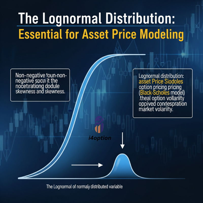
2. The Lognormal Distribution: Essential for Asset Price Modeling
While returns are often modeled as normal, asset prices themselves are usually modeled with a lognormal distribution. A variable is lognormally distributed if its logarithm is normally distributed. Stock prices can’t go negative (a key limitation of the normal distribution, which extends to negative infinity), so assuming lognormal price behavior makes sense. If continuous returns (log returns) are normal, then price = initial_price × e^(return) will be lognormal. The Black–Scholes option pricing model famously assumes that under risk-neutral conditions, an underlying asset’s future price follows a lognormal distribution. In practical terms, this means the distribution of a stock or index level is skewed to the right (a long right tail), since price is bounded by zero on the lower side but unbounded on the upside.
For example, consider the Nifty 50, currently around 250000. If we assume an annual volatility of ~15%, the Black–Scholes framework implies that Nifty’s price in one year is lognormally distributed with a certain mean and standard deviation (the mean drift would depend on risk-free rate under risk-neutral pricing). This lognormal model could estimate, say, the probability that Nifty is above 27,500 in one year or below 23,000 in one year. Traders use such projections to price options and structured products. Stock prices like TCS or Reliance are also often treated as lognormal in simulations – even if their short-term returns aren’t perfectly normal, lognormal is a reasonable model for prices given the no-negatives constraint. A key feature of lognormal models is that they handle multiplicative changes: for instance, a 10% drop on a ₹100 stock takes it to ₹90, and a subsequent 10% gain from ₹90 only brings it back to ₹99 (not ₹100). The distribution of outcomes is skewed such that large positive moves are possible (e.g. doubling in price), but negative moves are limited to -100%. This asymmetry naturally emerges under a lognormal assumption and aligns with how real stocks behave.
Illustrative lognormal distribution of asset prices. A lognormal curve skews to the right, reflecting that prices are bounded by zero on the downside but have potentially unlimited upside. Large gains are more probable than equally large losses (since losses are capped at -100%). In trading, assuming lognormal price behavior is common – it underlies the Black–Scholes model for options and ensures simulated prices can’t go negative. For example, a cheap stock doubling in price (+100%) is within the lognormal’s long tail, whereas the worst it can do is fall to zero (-100%).
In summary, modeling prices as lognormal is a staple for institutions, especially in derivatives pricing and risk modeling. It ensures no negative prices and aligns with the idea of compounding returns. NSE’s index options and stock option pricing models, for instance, are rooted in assumptions of lognormal underlying distributions (unless more complex models are used). Of course, like any model, lognormal is an approximation – actual price distributions for Nifty or Bank Nifty can deviate (showing heavier tails or skew than a pure lognormal). Still, lognormal is a very useful default starting point in trading models because of its tractability and its realistic reflection of positive-only prices.
3. The Binomial Distribution: Analyzing Discrete Trading Outcomes
The binomial distribution is a discrete distribution giving the probability of a certain number of “successes” in a fixed number of independent trials, when each trial has the same probability of success p. In trading, you can think of a “success” as any binary outcome of interest – e.g., a profitable trade (success) vs a losing trade (failure), or an event happening vs not happening. Many trading scenarios boil down to sequences of binary outcomes (win/lose, hit/miss). If you have a strategy that wins 60% of the time on each trade (p = 0.6) and you plan to take 10 trades, the binomial distribution can tell you the probabilities of getting exactly 0 wins, 1 win, 2 wins, … up to 10 wins out of those 10 trades. The two parameters defining a binomial distribution are n (number of trials) and p (success probability per trial).

For a concrete example, imagine a proprietary trading desk executes 5 intraday trades on Bank Nifty futures, with each trade having an estimated 70% chance of profit (perhaps based on historical performance). The probability that exactly 4 out of 5 trades are profitable is given by the binomial formula:
P(X=4) =(45 )x(0.7)2x(0.3)1,
which comes out to about 36.3%. Meanwhile, the probability that at least 4 trades are profitable (i.e. 4 or all 5) can be computed by summing the probabilities for 4 and 5 successes. A trader might use this to understand the odds of hitting a certain “win rate” over a day or week. For instance, “What are the chances I profit in at least 8 out of the next 10 trades?” – a binomial calculation can answer that. This is especially useful in quantitative backtesting: if a strategy has a win probability p per trade, one can estimate the distribution of total wins (and thus, with average profit per win and loss per loss, the distribution of total P/L) over many trades. It gives a sense of the variability in outcomes to expect purely from the randomness of wins and losses.
The binomial framework also underpins some option pricing models. The Binomial Options Pricing Model (BOPM) breaks an option’s life into discrete time steps and assumes the underlying price can move up or down by certain factors each step. After N steps, the number of up-moves in the price path follows a binomial distribution (with some risk-neutral probability q of an up-move each step). While this is used primarily for valuation (under risk-neutral probabilities rather than real-world p), it’s interesting that the lattice of possible underlying prices at expiry essentially comes from a binomial tree. For example, pricing a long-dated option on Nifty 50 via a multi-step binomial model involves averaging the payoff over a range of final outcomes that are generated by a binomial distribution of upward moves.
From a trading perspective, thinking in binomial terms reinforces the idea of each trade as a probability game. If you know (or estimate) your trade success probability, you can better manage expectations and risk. Even a 60% win-rate strategy will inevitably have losing streaks. The binomial distribution might tell you that the chance of, say, 3 or more losses in the next 5 trades is X%. This can prevent overreaction during a rough patch – it might just be a normal statistical fluctuation rather than a sign that the strategy has failed. Professional trading desks monitor such statistics to see if performance deviates significantly from expectation. For instance, if a trader with a long-term 60% win rate suddenly hits 10 losses in 12 trades, how unlikely is that under the binomial model? If it’s extremely unlikely, it might indicate something has changed in the strategy or market; if it’s not so unlikely, it might just be variance. In fact, institutional risk managers often use a binomial test to evaluate whether a string of losses is just bad luck or statistically significant.
In summary, the binomial distribution is a simple but powerful tool whenever we reduce trading outcomes to success/failure. Prop desks, HFT firms, and algorithmic traders use it implicitly to understand hit rates and the risk of sequences of wins/losses. It emphasizes that even with an “edge” (p > 0.5), outcomes in the short run are probabilistic. Only over many trials does the law of large numbers kick in, with the proportion of wins converging to the expected p. Seasoned traders thus think in terms of probabilities like “There’s an 80% chance I’ll be profitable on at least 15 of the next 20 trading days, given my past hit rate” rather than treating each trade as a sure bet.
4. The Poisson Distribution: Modeling Event Frequencies in Trading
The Poisson distribution is another discrete distribution, often used to model the number of times an event occurs in a fixed interval of time (or space), under the assumption that events happen independently and at a constant average rate. In trading, Poisson processes are frequently assumed for random event counts like order arrivals, trades, or even extreme moves. For example, an algorithmic trader might assume that the number of buy orders for Reliance Industries stock arriving in one second follows a Poisson distribution with some mean rate λ (lambda). If λ = 20 orders per second on average, a Poisson model can give the probability of seeing, say, 30 or more orders in a particularly busy second, or conversely, 0 orders in a quiet second. Similarly, one might model the number of new 52-week highs made by Nifty 50 stocks in a month using a Poisson distribution (e.g., if historically λ = 5 stocks per month hit new highs, what’s the probability that 10 do next month?).

One key property of Poisson processes is that if events follow a Poisson distribution for counts, the time between consecutive events follows an Exponential distribution. The exponential distribution is continuous and memoryless – it describes the probability distribution of waiting times between independent random events. In a high-frequency trading scenario, if we assume orders come in as a Poisson process, then the inter-arrival time (e.g., the gap in milliseconds between order arrivals) is exponentially distributed. For instance, suppose on the NSE, buy orders for Bank Nifty futures arrive at an average rate of 50 orders per second (λ = 50). The expected waiting time between orders is 1/λ = 0.02 seconds, and the distribution of actual waits is exponential. This means the probability that the wait time exceeds t seconds is exp(-50 * t). In practical terms, an HFT system might use this to anticipate how quickly it needs to react – if, on average, another order hits the book every 0.02s, a response latency of a few milliseconds might give a competitive edge before the next batch of orders arrives.
HFT firms and exchange microstructure models often start with Poisson assumptions because they make the math tractable. In fact, many theoretical order-book models assume arrivals of limit orders, market orders, and cancellations are independent Poisson processes (each with its own rate λ) to derive analytical results. Quants can then calibrate these rates from data. For example, they might observe that during the market open, orders arrive at a higher rate (λ surges), and around lunchtime, it slows – technically this violates the strict “constant λ” assumption of a Poisson process, but in short intervals under stable conditions, Poisson can be a reasonable approximation for random order arrivals. Market makers use these models to estimate fill probabilities: e.g., “What’s the probability I get 5 or more buy orders hitting my quotes in the next second?” – assuming a Poisson(λ) for buy orders, one can compute that quickly. In general, Poisson processes offer a framework for traders to model the randomness and frequency of discrete events in markets
It’s important to note that real-world data often shows over-dispersion or clustering, meaning a simple Poisson model might not perfectly fit. For example, empirical studies of high-frequency data find that order arrivals are not truly independent – there are bursts of activity and lulls, which violate the constant λ assumption. A sudden news release might cause a flood of orders (clustering in time), followed by quiet periods. Researchers have observed that assuming homogeneous Poisson arrivals underestimates the frequency of rapid-fire bursts and overestimates the frequency of perfectly steady flows. In other words, real order flow often has self-exciting behavior (one spike of activity begets more activity shortly after) rather than perfectly random independent arrivals. This has led to more advanced models (like Hawkes processes, which are essentially “infectious” Poisson processes where an event increases the short-term likelihood of follow-up events).
Nevertheless, many trading algorithms and models still use Poisson processes as a building block, thanks to their simplicity. They may then layer on adjustments for time-varying rates or clustering as needed. For example, an exchange might assume baseline Poisson arrivals for orders but allow the rate λ to be a function of time of day (higher in volatility periods). Or a risk model might simulate rare jump events (like a market-wide sudden drop) as a Poisson process on top of continuous price fluctuations (a jump-diffusion model). Even if not perfect, the Poisson distribution gives a first-cut insight into random event frequencies that is valuable. It’s also widely used in risk management to model event counts: think of the number of credit defaults in a bond portfolio (often modeled via Poisson), or the count of 3σ+ large moves in a year for an index (if historically ~2 such moves per year for Sensex, one might model extreme jumps per year as Poisson with λ ≈ 2). Traders and analysts use these to price instruments that are sensitive to event frequency; for instance, some options and structured products account for the possibility of jumps occurring as a Poisson process superimposed on continuous price changes.
To summarize, the Poisson distribution (and its continuous-time cousin, the exponential) are invaluable for modeling random discrete events in trading. HFT operations, exchange analysts, and quants use them to model everything from trade arrivals and order flow to the frequency of big market moves or news events. In Indian markets, an analyst might estimate that on average 1000 trades per minute occur on Nifty futures, then use Poisson math to figure the probability of a 1500-trade frenzy in a particular minute (perhaps during a sudden volatility spike). As always, one must be cautious: if events aren’t truly independent or rates shift over time, a basic Poisson model’s predictions can break down. Markets often exhibit feedback loops (e.g., heavy trading volume begets even more volume as algorithms react), which a simple Poisson can’t capture. Advanced desks account for this by dynamically updating rates or using self-exciting process models – but the foundation remains understanding the simple Poisson process and distribution.
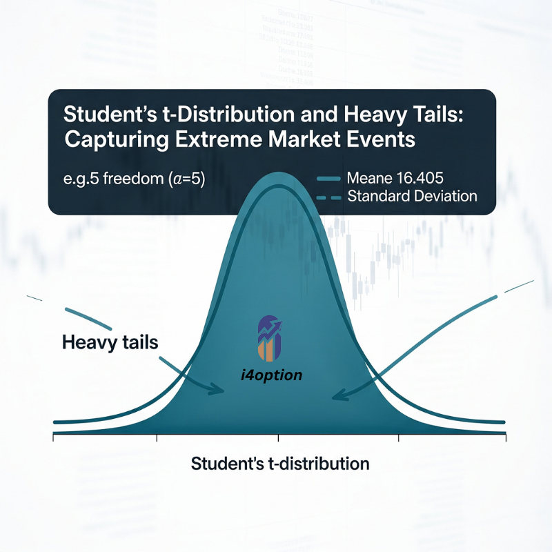
5. Student’s t-Distribution and Heavy Tails: Capturing Extreme Market Events
As mentioned earlier, financial return distributions often have fat tails – extreme outcomes happen more frequently than the normal distribution would suggest. This has led institutional traders and risk managers to use heavy-tailed distributions to model returns and risk. A heavy-tailed distribution allocates more probability to far-from-the-mean events (the tail ends of the distribution) compared to a normal curve. One popular example is the Student’s t-distribution, which looks similar to a normal bell curve around the center but has much thicker tails. The t-distribution is characterized by degrees of freedom (df): the lower the df, the heavier the tails (i.e., more probability in the extremes). In fact, as df → ∞, the t-distribution converges to normal; but with small df (like 3, 4, 5), it better captures those outlier moves that we see in markets.
Institutional trading desks often prefer using a t-distribution (or a variant of it) for modeling portfolio returns or asset returns when computing risk metrics like Value-at-Risk (VaR). A normal-based VaR can severely underestimate the risk of large losses because it underweights the tail events. For example, if we look at 5-year daily returns of Nifty 50, a normal fit might drastically understate the frequency of 3% or 4% daily moves. A Student’s t distribution with an appropriate df could fit the data’s heavier tails more accurately, thus predicting a higher probability for, say, a -5% day than the normal model would. Research has shown that for many markets (including emerging markets like India), a heavy-tailed model (t or a skewed-t) fits return distributions better than a normal model. In one study of an emerging market, the skewed Student’s t provided a superior fit over the normal for modeling returns and volatility– a pattern likely true for Indian markets as well, where large moves relative to volatility occur due to regime shifts, global events, etc. In fact, statistical tests on Nifty data almost always indicate excess kurtosis (a tall peak and fat tails) and reject the hypothesis of normality.
Let’s consider a practical use case: A risk manager at an Indian bank is estimating the 1-day 99% VaR for a portfolio of Nifty and Bank Nifty futures. Using a normal distribution for returns might give a VaR number (the loss threshold that’s exceeded only 1% of the time) that doesn’t fully account for events like the 2020 pandemic crash. If instead they assume a Student’s t-distribution with, say, 4 degrees of freedom, the 99th percentile loss will be larger – indicating more risk – because the model expects a higher likelihood of extreme drops. In trading terms, this is a more conservative approach that acknowledges “worst-case” scenarios happen more often than the naive normal model predicts. Many hedge funds and prop desks similarly use heavy-tailed assumptions for stress-testing: e.g., “What’s the probability our portfolio loses more than 5σ in a day?” Under a normal, it’s essentially 0%, but under a t-dist with df=3 it might be, say, 0.5% – not huge, but not zero either. That difference can justify holding extra capital or hedges for tail risk. As the saying goes, “Markets can remain irrational longer than you can remain solvent,” and part of that irrationality is the occurrence of outsized moves that a simplistic model might call impossible. By using fat-tailed models, traders seek to avoid underestimating that risk, and sometimes even to profit from mispriced tail events (through tail-risk hedging strategies or options).
Aside from the Student’s t, traders and quants have explored other heavy-tailed distributions: Pareto distributions (power-law tails, useful for extreme losses or wealth distributions), Cauchy distribution (so heavy-tailed it has infinite variance; rarely used directly, but a theoretical extreme case), Levy distribution (a stable distribution with a heavy right tail, used in some fractal price models), and alpha-stable distributions (a family generalizing normal and Cauchy, allowing heavy tails and skew). These are more niche, but for example, some advanced option pricing models use a variance-gamma or hyperbolic distribution for underlying returns to better fit the implied volatility smile – those distributions are also heavy-tailed relative to normal. In academic research on Indian markets, you’ll even find attempts to fit stable Paretian distributions to returns; one analysis of Nifty returns via alpha-stable laws found the return series had much thicker tails than normal, again reinforcing that a normal model is too thin-tailed for Nifty 50.
For day-to-day trading, the most straightforward heavy-tailed adjustment is to use Student’s t. It’s implemented in many software packages, and one can calibrate the degrees of freedom by looking at the historical kurtosis of returns. High-frequency trading algorithms might also implicitly account for heavy tails – for instance, algorithms may have separate logic for “tail events” (like circuit-breaker days or flash crashes), recognizing that those aren’t as improbable as a normal distribution would suggest. Options traders, too, are keenly aware of heavy tails: the very existence of the volatility skew/smile in implied volatilities is a reflection that the market’s implied distribution of returns is not normal but skewed and heavy-tailed. A far out-of-the-money index put has a higher implied vol than an at-the-money option, effectively indicating the market is assigning extra probability to crash-like moves (heavy left tail) compared to the normal assumption.
To wrap up, heavy-tailed distributions are crucial for capturing the risk of extreme market moves. Institutional players use them to avoid being lulled into a false sense of security by the bell curve’s thin tails. The Student’s t-distribution with moderate degrees of freedom is a common choice, balancing complexity and realism. It acknowledges that while everyday volatility might be modest, rare events like 5σ or 6σ moves do happen and should not be ignored. In the Indian context, events such as sudden government policy announcements, global market contagion episodes, or a major corporate default can all cause heavier-tail behavior in indices – those who model that possibility are a step ahead in risk management.
Histogram of daily log returns for Nifty 50 ( refer earlier articles) and Bank Nifty (blue bars), overlaid with a fitted normal curve (red line). Notice the empirical distribution has a sharper peak and much fatter tails than the normal bell curve. This is evidenced by very high kurtosis values (e.g., Nifty’s excess kurtosis ≫ 0) and a near-zero p-value on the Jarque–Bera test for normality. In other words, actual return distributions deviate significantly from normality, exhibiting heavy tails (far more frequent extreme moves than Gaussian theory would predict).
Conclusion: Embracing Probabilistic Thinking in Modern Markets
Probability distribution functions provide the mathematical backbone for quantifying uncertainty in trading. Whether you are a day trader on NSE or a quant at a hedge fund, thinking in terms of distributions – rather than single-point predictions – is key to navigating markets. In this post we introduced various distributions and how they’re applied in trading: Normal (the classic but thin-tailed bell curve underpinning many basic models), Lognormal (for prices bounded by zero, critical in options pricing), Binomial (for binary outcomes like trade wins/losses or up/down moves), Poisson/Exponential (for modeling random event counts and timing, especially in HFT and order flow), and heavy-tailed distributions like Student’s t (to account for the market’s propensity for extreme moves). Each of these has its place in a trader’s toolkit:
- Institutional traders and risk managers might start with normal assumptions for convenience but then adjust for reality with heavy-tailed models. They frequently use t-distributions or empirically derived distributions for stress tests and VaR calculations, ensuring they’re not caught off guard by the fat tails that the bell curve underestimates.
- High-Frequency Trading firms rely on Poisson and exponential models for microstructure (e.g. modeling order arrivals and trade counts) while also recognizing when those models break down (for instance, during a sudden volume spike or news event that violates the independent Poisson assumption).
- Proprietary trading desks use binomial thinking to evaluate strategy performance and risk of ruin – treating each trade or each day as part of a distribution of outcomes rather than a guaranteed profit or loss. This helps in setting realistic expectations and risk limits (e.g., “what’s the probability of X losing days in a row?”).
- Options traders implicitly work with probability distributions every day – an option’s price essentially reflects the market’s consensus distribution for the underlying’s future price. Thus, understanding how altering distributional assumptions (normal vs skewed vs fat-tailed) affects option values is crucial. For example, pricing Nifty options assuming a lognormal distribution vs a heavy-tailed distribution will yield different risk metrics and can explain why deep OTM options carry a volatility skew.
One recurring lesson is that no single distribution is perfect for markets. Markets exhibit features like volatility clustering, regime changes, and anomalies that challenge simple static distribution assumptions. In practice, traders often use hybrid approaches: perhaps assume near-normal behavior for small day-to-day moves but incorporate Poisson-driven jumps for large moves (the basis of jump-diffusion models), or use actual historical return distributions (empirical distribution) directly in simulations. The goal is to be approximately right rather than exactly wrong – having a rough distributional understanding is better than assuming deterministic outcomes.
By grounding our discussion in examples like Nifty and Sensex moves, or the frequency of trades/orders, we see that these concepts are not abstract math but daily realities. Questions like “What is the chance Nifty falls 3% tomorrow?”, “How many stocks might hit upper circuit in a year?”, or “How likely am I to have 4 losing trades in a row?” are all answered with probability distributions. A deep appreciation of these probabilities is part of what separates professional traders from gamblers. Professionals continuously weigh risk and reward in probabilistic terms, often speaking in terms of probability-adjusted outcomes or odds of scenarios rather than certainties.
In conclusion, probability functions and distributions form the bedrock of quantitative trading and risk management. They enable traders to encode uncertainty, make data-driven decisions, and survive the randomness inherent in markets. As we continue in this series, we will build on this foundation – leveraging distributional thinking in more advanced trading concepts and exploring how these probabilities connect to real market pricing and strategy. Whether you’re analyzing Nifty’s volatility, crafting an options strategy on Bank Nifty, or testing an algorithm on TCS stock, remember: think in probabilities and distributions, not certainties. It’s a mindset that will serve you well in the unpredictable world of markets. Happy trading!
Key Probability Distributions in Trading – A Comparative Overview
| Distribution Name | Type | Key Characteristics | Primary Application in Trading | Illustrative Indian Market Example |
| Normal | Continuous | Symmetric bell curve; defined by mean & std dev | Returns modeling, basic volatility analysis | Nifty 50 daily returns, TCS stock daily moves |
| Lognormal | Continuous | Right-skewed; bounded by zero; logarithm is normal | Asset price modeling, options pricing | Nifty 50 future price, Reliance Industries stock price |
| Binomial | Discrete | Fixed trials, independent, binary outcomes, constant p | Strategy win rates, risk of ruin | Prop desk Bank Nifty futures trades, backtesting win/loss sequences |
| Poisson | Discrete | Event counts in fixed interval; constant average rate | Order flow analysis, event frequency | Number of buy orders for Reliance Industries per second, Nifty futures trade volume spikes |
| Student’s t | Continuous | Symmetric with heavier tails than Normal; df parameter | Risk management, extreme event modeling | 1-day 99% VaR for Nifty/Bank Nifty futures portfolio, fitting fat tails in Nifty returns |
Hope you are enjoying this statistical series. Please let me know If you think we need a detailed explanation of any of above above-listed probability distribution functions.