When discussing market volatility or risk in stocks and indices, such as the Nifty 50, two key statistical concepts often arise: standard deviation and the normal distribution. In this article, we’ll break down what these terms mean in simple terms, how to calculate measures like mean, variance, and standard deviation for stock market data, and what it means when traders talk about “1 SD, 2 SD, 3 SD” moves. We’ll also look at a case study using one year of daily Nifty 50 index data (FY 2024–25) to see if its daily returns follow a normal distribution or not.

Mean and Variance: Measuring Average and Dispersion

Before diving into standard deviation, we need to understand mean and variance – the building blocks of standard deviation.

• Mean (Average): The mean is the simple average of a set of numbers. To get the mean, you add up all the values and divide by the number of values. For example, if we have daily returns of +1%, +2%, and -1%, the mean return is (1 + 2 + (-1)) / 3 = 0.67%. This is the expected value around which other values tend to cluster.
• Deviation from the Mean: Each data point will differ from the mean by some amount – this difference is called a deviation. Some deviations are positive (if the data point is above the mean) and some are negative (if below the mean). If you average up all raw deviations, they’d cancel out to zero by definition of the mean. So instead, we consider the squared deviations to measure overall spread in a positive way.
• Variance: The variance is the average of the squared deviations from the mean. In other words, for each data point, calculate (value – mean), square each of those differences, then take the average of those squared differences. Squaring ensures that negative and positive deviations don’t cancel out, and it gives more weight to larger differences. The formula for variance for a set of values.                                                                                                
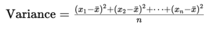
  (If you are using a sample of data, typically you divide by n-1 instead of n for an unbiased estimate, but the concept is the same.)

Variance gives us a measure in squared units (for example, if returns are in percentage, variance is in “percentage squared”), which isn’t very intuitive to interpret. This is where standard deviation comes in.

What Is Standard Deviation?

Standard deviation (SD) is simply the square root of the variance. By taking the square root, we bring the number back to the original units of the data, making it much easier to interpret. In plain language, standard deviation tells us, on average, how far data points tend to be from the mean. It’s a measure of spread or volatility in the same units as the data itself.

For example, if the daily closing prices of a stock have a standard deviation of 2%, that means most daily moves are around 2% away from the average move. A higher standard deviation means data points (or price returns) are more spread out (more volatile), while a lower standard deviation means they are tightly clustered around the mean (more stable). In finance, standard deviation is one of the most common metrics for market volatility and risk. A larger SD implies a riskier asset, since price swings can be larger, whereas a smaller SD implies a steadier asset price movement.

To calculate standard deviation step by step:

1. Calculate the mean of your data set (as described earlier).
2. Find the deviation of each data point from the mean (each value minus the mean).
3. Square each deviation.
4. Find the average of these squared deviations – that gives you the variance.
5. Take the square root of the variance – that gives you the standard deviation.

In formula form, the standard deviation is often denoted by the Greek letter sigma  ( σ). Using the same terms as above,

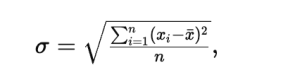
which is just the square root of the variance formula. (Again, if using a sample, you would use n-1 in the denominator.) The result sigma is in the same unit as x_i; in our case, it is % (daily return % number)

So, if we were looking at daily returns of a stock or index, sigma would be in “% per day”. For instance, suppose the Nifty 50 index has an average daily return of ~0.02% and a standard deviation of ~0.9% per day (we’ll see actual numbers shortly). That 0.9% daily SD means a typical daily move is around 0.9% up or down from the mean. Some days will be calmer (closer to zero change), and some will be more volatile (several percentage points move), but about two-thirds of days should fall within roughly ±0.9% if the distribution is normal (more on that next).

The Normal Distribution (“Bell Curve”) and the Empirical Rule

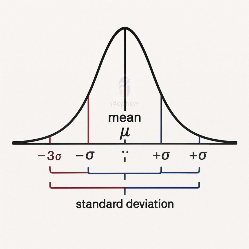
When people refer to “normal distribution”, they mean the well-known bell-shaped curve in statistics. A normal distribution is a symmetric curve centered around the mean, and its shape is determined by the mean (center) and standard deviation (spread). Many natural phenomena and measurement errors tend to follow this pattern. In a perfect normal distribution, most values cluster around the mean (forming the peak of the bell curve), and the probability of values further from the mean tapers off equally in both the positive and negative direction.

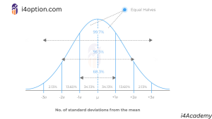
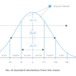
Figure: The bell curve of a normal distribution illustrating the empirical 68–95–99.7% rule. Each colored band shows one standard deviation increment from the mean (center). Approximately 68% of data points lie within ±1 SD, ~95% within ±2 SD, and ~99.7% within ±3 SD of the mean.

In a normal distribution, there is a very neat rule of thumb known as the Empirical Rule (68–95–99.7% rule). It states that for a normal dataset:

• Approximately 68% of the data will fall within ±1 standard deviation of the mean.
• About 95% will fall within ±2 standard deviations.
• Around 99.7% will fall within ±3 standard deviations of the mean.

This is where terms like “1 SD, 2 SD, 3 SD” come into play. If a trader says “today was a 2-sigma move,” they mean the day’s price change was 2 standard deviations away from the average, which, under a normal assumption, should be a rather unusual event (only ~5% of occurrences are beyond ±2 SD). A “3-sigma” move is even more extreme (only ~0.3% of outcomes expected beyond ±3 SD – in other words, very rare under the normal curve). These benchmarks give a quick sense of how extraordinary a given price move is compared to typical daily volatility.

However, financial returns don’t always perfectly follow a normal distribution. The normal curve is a useful approximation, but real market data often shows skewness (asymmetry) or “fat tails” (more extreme events than predicted by a normal curve). Fat tails mean those 0.3% probability extreme moves happen more often than 0.3% in reality – something important for risk management. We’ll explore this point with an example from the Nifty 50.

Case Study: Do Nifty 50 Daily Returns Follow a Normal Distribution?

Let’s put this into practice with a real-world example. We examined daily closing data for the Nifty 50 index over the financial year 2024–25 (April 1, 2024 through March 31, 2025). We calculated the daily percentage return (today’s close vs yesterday’s close) for each trading day in that year, then computed the mean and standard deviation of those daily returns. Here’s what we found:

• Mean daily return: Approximately +0.02%. In other words, the average daily move was slightly positive (as markets tend to drift upward over the long term, a tiny positive daily mean is expected).
• Standard deviation of daily returns: Approximately 0.89%. This means on an average day, the Nifty’s change was around ±0.9%. We can think of this as the “typical” daily volatility. Some days are bigger moves, some are smaller, but 0.9% is the scale of a usual day’s fluctuation.

Now, if Nifty’s daily returns were perfectly normally distributed with mean ~0 and σ ~0.89%, we would expect about 68% of days to be within ±0.89% (i.e., between -0.89% and +0.89%), about 95% of days between ±1.78% (twice 0.89%), and only 0.3% of days to move beyond ±2.67% (three times 0.89%).

Let’s compare this theoretical expectation with what actually happened in FY 2024–25:

• Within ±1 SD (≈ ±0.9%): We observed roughly 77% of days had daily returns in this range. That’s actually more than the 68% expected from a perfect normal distribution. In other words, small daily changes happened even more frequently than the normal model would predict – the bell curve for Nifty returns is a bit peaked (taller in the middle) compared to a standard normal.
• Within ±2 SD (≈ ±1.8%): About 96% of days fell inside this band, which is very close to the 95% expected in a normal distribution. So up to about ±2% moves, reality and the normal model are in fairly good agreement.
• Beyond ±3 SD (more than ~±2.7% move): We had a few outlier days. In fact, 4 trading days (about 1.6% of the year’s sessions) saw moves beyond 3 standard deviations (two of those were sharp drops around -3% to -6%, and two were big gains above +3%). Ideally, a normal distribution would expect only 0.3% of days to be that extreme – which would be roughly 0.7 days in a year (obviously you can’t have 0.7 of a day, but think of it as “once in several years”). We got 4 such extreme days in just this one year. This is a sign of “fat tails” – extreme events occurred more often than the normal curve predicts. These rare but significant jolts are what make real financial data riskier than a naive normal assumption might imply.

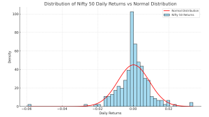
Figure: Distribution of Nifty 50 daily returns for FY 2024–25 (blue histogram), compared to an ideal normal distribution (red curve) with the same mean and standard deviation. We can see the actual distribution is roughly bell-shaped, but it has a higher peak (more days with tiny moves around 0) and slightly fatter tails (a few more extreme moves) than the normal curve suggests. The leftmost bar corresponds to a ~-5.9% day, a significant outlier.

Looking at the above histogram, the overall shape is somewhat bell-curved – indeed, daily returns of indices often approximate a normal distribution in the center. Many days are small changes clustered near 0%. However, the peak is taller and narrower than a perfect Gaussian, and the histogram has outliers that make the tails heavier. For example, that one day with nearly -6% drop is far out on the left, well outside the red curve’s main range. The normal curve (red line) underestimates the probability of such an event. This aligns with financial statistics research: over longer periods or large samples, stock market returns are not perfectly normal and tend to exhibit leptokurtosis – a fancy term meaning a high peak and fat tails compared to a normal distribution. In plain English, there are more extremely quiet days and more extremely wild days than the ideal bell curve would suggest.

So, does Nifty 50 follow a normal distribution?

Not exactly, but it’s not a terrible first approximation for moderate moves. The one-year period we studied had returns that were roughly symmetric around the mean and mostly fell in a bell-shaped pattern. For many practical purposes (like basic risk estimates), assuming a normal distribution might be okay for that timeframe. But the differences are important: the market had slightly more stability on most days (more small fluctuations) and a higher chance of extreme swings than a true normal distribution would predict. These “fat tail” phenomena mean risk can be underestimated if one blindly uses normal assumptions. In fact, a rigorous statistical test on a longer dataset often rejects normality – for example, one 5-year study confirmed that Nifty 50 daily returns did not pass normality tests, and suggested using distributions with heavier tails for better modeling.

Conclusion

Understanding standard deviation gives traders and investors a quantitative handle on market volatility – it answers “how much do prices typically deviate from the average?” We also introduced the normal distribution (bell curve) as a useful model for randomness, along with the 68–95–99.7% empirical rule that helps contextualize 1 SD, 2 SD, and 3 SD moves. When applying these concepts to real stock market data like the Nifty 50, we find reality is close to but not perfectly normal. Most days might behave in a well-behaved way, but the market can surprise us with outsized moves more often than the ideal bell curve predicts.

For the general reader or retail trader, the key takeaways are: standard deviation is a crucial number for gauging risk, and phrases like “1 sigma move” refer to how unusual a price change is in volatility terms. Just remember that the market’s “bell curve” has a propensity for surprises at the tails. By being aware of these statistics, you can better appreciate both the typical market rhythm and the possibility of those rare, volatile days that aren’t as rare as a textbook normal distribution might suggest!

Video: Watch the video of this concept, shared on the YouTube channel